How to Fine-Tune Mistral 7B on Your Own Data With LoRA: A Complete Guide for Local AI

You can fine-tune a powerful 7-billion parameter language model like Mistral 7B on a consumer-grade GPU with as little as 12-16GB of VRAM, in under two hours. This is not hyperbole; it’s the reality brought by Low-Rank Adaptation (LoRA) and efficient quantization techniques. Forget weeks of cloud GPU rentals and five-figure bills. This guide will walk you through the precise, step-by-step process of customizing Mistral 7B with your own data, entirely locally, democratizing advanced AI for every developer and tinkerer.

Image: Mistral AI

Prerequisites: What You Need Before Starting

Fine-tuning Mistral 7B with LoRA locally requires a few key components. While LoRA significantly reduces VRAM usage, a capable GPU is still essential. We recommend a Linux-based system for the smoothest experience, though macOS (with Apple Silicon) and Windows (with WSL2 and NVIDIA GPUs) are also viable.

• Minimum Hardware:
  • GPU: NVIDIA RTX 3060 (12GB VRAM) or equivalent. Apple M1/M2/M3 chip with at least 16GB unified memory.
  • RAM: 32GB system RAM.
  • Storage: 100GB free SSD space.
• Recommended Hardware:
  • GPU: NVIDIA RTX 4070 (12GB VRAM), RTX 3090 (24GB VRAM), or RTX 4090 (24GB VRAM). Apple M1 Pro/Max/Ultra or M2 Pro/Max/Ultra with 32GB+ unified memory.
  • RAM: 64GB+ system RAM.
  • Storage: 200GB+ free NVMe SSD space for faster data loading.
• Software:
  • Operating System: Ubuntu 22.04+ (recommended), macOS Sonoma+, Windows 10/11 with WSL2.
  • Python: Python 3.10 or newer.
  • Package Manager: pip.
  • GPU Drivers: Latest NVIDIA drivers for CUDA, or Apple’s Metal Performance Shaders (MPS) for macOS.
  • Frameworks: PyTorch (2.0+), Transformers, Accelerate, PEFT (Parameter-Efficient Fine-tuning), TRL (Transformer Reinforcement Learning).

Ensure your environment is set up with CUDA (for NVIDIA GPUs) or MPS (for Apple Silicon) to leverage GPU acceleration effectively. This will drastically reduce training times compared to CPU-only execution.

Step 1: Prepare Your Environment and Install Dependencies

The first step involves setting up a dedicated Python environment and installing all necessary libraries. It’s crucial to use a virtual environment to avoid conflicts with other Python projects. This isolation ensures reproducibility and prevents version conflicts with other machine learning projects you might be working on simultaneously.

Before proceeding, verify your CUDA installation (for NVIDIA GPUs) by running nvidia-smi to check GPU availability and VRAM. For macOS users, verify Metal Performance Shaders support with python -c "import torch; print(torch.backends.mps.is_available())". This initial verification prevents wasted setup time if your environment isn’t properly configured for GPU acceleration.

# Create a virtual environment
python3 -m venv lora-finetune-env
source lora-finetune-env/bin/activate

# Install PyTorch (CUDA 12.1 example - adjust for your CUDA version or MPS)
# For NVIDIA CUDA:
pip install torch torchvision torchaudio --index-url https://download.pytorch.org/whl/cu121
# For Apple Silicon (macOS):
# pip install torch torchvision torchaudio

# Install Hugging Face libraries
pip install transformers peft accelerate trl bitsandbytes datasets

# Verify installation (optional)
python -c "import torch; print(f'PyTorch version: {torch.__version__}'); print(f'CUDA available: {torch.cuda.is_available()}')"

If torch.cuda.is_available() returns False, double-check your GPU drivers and PyTorch installation. For Apple Silicon, torch.backends.mps.is_available() should return True.

Step 2: Curate and Format Your Dataset

The quality of your fine-tuning data is absolutely paramount. This cannot be overstated. For instruction-following models like Mistral 7B, your data should ideally be in an instruction-response format. A common format is JSONL (JSON Lines), where each line is a JSON object representing one training example. The model will only be as good as the data you feed it during fine-tuning, so invest time in data curation and validation.

Data preprocessing is equally important. Remove duplicate entries, ensure consistency in formatting, validate that responses are accurate and relevant, and eliminate any personally identifiable information (PII) or sensitive data. A dataset of 500 high-quality examples will typically outperform a dataset of 5000 mediocre examples. Consider having domain experts review at least 10% of your dataset to catch quality issues early.

[
    {"instruction": "What is the capital of France?", "response": "Paris."},
    {"instruction": "List 3 benefits of exercise.", "response": "Improved cardiovascular health, increased strength, better mood."},
    // ... more examples
]

For chat-based models, you might format it as a series of turns:

[
    {"messages": [{"role": "user", "content": "Hello, how are you?"}, {"role": "assistant", "content": "I'm doing great, thanks for asking!"}]},
    // ...
]

Save your dataset as train_data.jsonl. For optimal results, aim for at least 500-1000 high-quality examples. More is generally better, but quality trumps quantity. Avoid noisy, irrelevant, or repetitive data.

Step 3: Load Mistral 7B and Configure LoRA

Now, we’ll load the base Mistral 7B model and configure the LoRA adapters. LoRA works by adding small, trainable matrices (adapters) to the existing model layers, rather than modifying the entire model. This drastically reduces the number of trainable parameters and VRAM footprint.

from transformers import AutoModelForCausalLM, AutoTokenizer, BitsAndBytesConfig
from peft import LoraConfig, get_peft_model, prepare_model_for_kbit_training
import torch

# Configuration for 4-bit quantization (optional, but recommended for consumer GPUs)
nf4_config = BitsAndBytesConfig(
    load_in_4bit=True,
    bnb_4bit_quant_type="nf4",
    bnb_4bit_use_double_quant=True,
    bnb_4bit_compute_dtype=torch.bfloat16 # or torch.float16 for older GPUs
)

# Load base Mistral 7B model with quantization
model_id = "mistralai/Mistral-7B-v0.1" # Or Mistral-7B-Instruct-v0.2 for instruction-tuned base
model = AutoModelForCausalLM.from_pretrained(
    model_id,
    quantization_config=nf4_config,
    device_map="auto" # Distributes model across available GPUs/CPU
)
model.config.use_cache = False
model.config.pretraining_tp = 1

# Load tokenizer
tokenizer = AutoTokenizer.from_pretrained(model_id, trust_remote_code=True)
tokenizer.pad_token = tokenizer.eos_token
tokenizer.padding_side = "right" # Important for training

# Prepare model for k-bit training (required for 4-bit/8-bit LoRA)
model = prepare_model_for_kbit_training(model)

# LoRA configuration
lora_config = LoraConfig(
    r=16, # Rank of the update matrices. A smaller `r` means fewer trainable parameters. Common values are 8, 16, 32, 64.
    lora_alpha=32, # LoRA scaling factor. Adjusts the magnitude of the updates. Typically twice `r`.
    lora_dropout=0.05, # Dropout probability for LoRA layers.
    bias="none", # Type of bias to train: "none", "all", or "lora_only". "none" is common for LLMs.
    task_type="CAUSAL_LM", # Specifies the task.
    target_modules=["q_proj", "k_proj", "v_proj", "o_proj", "gate_proj", "up_proj", "down_proj"] # Modules to apply LoRA to. These are common for Mistral.
)

# Apply LoRA to the model
model = get_peft_model(model, lora_config)

# Print trainable parameters
model.print_trainable_parameters()

The model.print_trainable_parameters() output should show that only a small percentage (typically <1%) of the total parameters are being trained, demonstrating LoRA's efficiency.

Step 4: Configure and Run the Trainer

With the data formatted and the model prepared, we can now set up the training arguments and start the fine-tuning process using Hugging Face’s Trainer API. This step integrates our dataset with the LoRA-enabled Mistral 7B model. The SFTTrainer (Supervised Fine-Tuning Trainer) is optimized for causal language modeling and handles many technical details internally, making it significantly simpler than manual training loops.

Before launching training, ensure you have sufficient disk space for checkpoints. With 3 epochs and default settings, expect 2-4GB of checkpoint storage. Monitor system temperature and VRAM utilization during the first few steps to catch potential stability issues early. Most modern GPUs can safely operate at 80-90°C for extended periods, but throttling or crashes will occur beyond that threshold.

from datasets import load_dataset
from trl import SFTTrainer
from transformers import TrainingArguments

# Load your dataset
dataset = load_dataset("json", data_files="train_data.jsonl", split="train")

# Define formatting function for SFTTrainer
def formatting_prompts_func(example):
    output_texts = []
    for i in range(len(example['instruction'])):
        text = f"### Instruction:\n{example['instruction'][i]}\n\n### Response:\n{example['response'][i]}"
        output_texts.append(text)
    return output_texts

# Training arguments
training_arguments = TrainingArguments(
    output_dir="./results", # Directory to save checkpoints and logs
    num_train_epochs=3, # Number of training epochs. Adjust based on dataset size and model convergence.
    per_device_train_batch_size=4, # Batch size per GPU/device. Adjust based on VRAM.
    gradient_accumulation_steps=2, # Accumulate gradients over multiple steps to simulate larger batch size.
    optim="paged_adamw_8bit", # Optimizer. paged_adamw_8bit is memory-efficient.
    save_strategy="epoch", # Save checkpoint every epoch.
    logging_steps=10, # Log training metrics every 10 steps.
    learning_rate=2e-4, # Learning rate. Common range 1e-5 to 5e-4.
    fp16=False, # Set to True if your GPU supports FP16 (often faster).
    bf16=True, # Set to True if your GPU supports BF16 (better numerical stability, RTX 30xx/40xx series).
    max_grad_norm=0.3, # Maximum gradient norm. Helps prevent exploding gradients.
    max_steps=-1, # Set to -1 to train for num_train_epochs.
    warmup_ratio=0.03, # Percentage of total steps to use for linear warmup.
    lr_scheduler_type="constant", # Learning rate scheduler type.
    report_to="tensorboard", # Report metrics to TensorBoard for visualization.
    disable_tqdm=False, # Enable tqdm progress bar.
)

# Initialize SFTTrainer
trainer = SFTTrainer(
    model=model,
    train_dataset=dataset,
    peft_config=lora_config,
    max_seq_length=512, # Maximum sequence length. Adjust based on your data and VRAM.
    tokenizer=tokenizer,
    formatting_func=formatting_prompts_func, # Use the custom formatting function
    args=training_arguments,
)

# Start training
trainer.train()

# Save the fine-tuned adapter
trainer.model.save_pretrained("./fine_tuned_mistral_lora")
tokenizer.save_pretrained("./fine_tuned_mistral_lora")

Monitor the training process via the console output and TensorBoard (if configured) for loss convergence. Adjust hyperparameters like learning_rate, num_train_epochs, and per_device_train_batch_size as needed. Common issues include out-of-memory errors (reduce batch size, gradient accumulation steps, or max_seq_length) or models not learning (check dataset quality, learning rate). Loss should steadily decrease over epochs; if it plateaus or increases, your learning rate is likely too high or your data has quality issues. Training loss between 0.5-2.0 is typical for LLM fine-tuning, depending on task complexity.

Step 5: Load and Test Your Fine-Tuned Model

After training completes, you can load your fine-tuned model and test it on sample inputs to evaluate its performance before deploying.

from transformers import AutoModelForCausalLM, AutoTokenizer, TextGenerationPipeline
from peft import AutoPeftModelForCausalLM

# Load the fine-tuned adapter
model = AutoPeftModelForCausalLM.from_pretrained(
    "./fine_tuned_mistral_lora",
    device_map="auto"
)
model.eval() # Set to evaluation mode

# Load tokenizer
tokenizer = AutoTokenizer.from_pretrained("./fine_tuned_mistral_lora")

# Create a text generation pipeline
pipeline = TextGenerationPipeline(
    model=model,
    tokenizer=tokenizer,
    device_map="auto"
)

# Test with a sample prompt
prompt = "### Instruction:\nWhat is machine learning?\n\n### Response:"
response = pipeline(prompt, max_new_tokens=256, temperature=0.7, top_p=0.9)
print(response[0]["generated_text"])

Compare the fine-tuned model’s outputs against the base Mistral 7B to see the improvement. Also test edge cases and out-of-distribution inputs to gauge robustness. If the model’s responses are not satisfactory, you may need to: (1) collect and add more domain-specific training examples, (2) adjust hyperparameters and retrain, or (3) increase LoRA rank for greater capacity. This iterative process is normal and expected.

Deployment and Integration

Once satisfied with your fine-tuned model, you can deploy it for inference. For production use, consider using Ollama for local inference, which streamlines model loading and API serving. Alternatively, you can wrap your model with FastAPI for a REST API or integrate it directly into your application. Remember to merge the LoRA adapters with the base model for production deployment to simplify model distribution and reduce latency. Use model.merge_and_unload() to create a merged model checkpoint.

Common Issues and Troubleshooting

CUDA Out of Memory (OOM): The most frequent issue. Solutions include reducing per_device_train_batch_size (e.g., from 4 to 2), increasing gradient_accumulation_steps, reducing max_seq_length, or using gradient checkpointing with gradient_checkpointing=True in the model configuration.

Model Not Learning / Loss Not Decreasing: Check your learning rate (try 1e-4 to 5e-4 range), validate dataset quality and format, ensure no data leakage between train and test sets, and verify the model is actually being updated (inspect model parameters before and after one step).

Training Crashes Mid-Epoch: Likely a data formatting issue. Validate your JSONL file, ensure all samples have required fields, and test with a small subset (100 examples) first to isolate the problematic sample.

Performance Tuning: Squeezing More Out of Your Local Setup

Image: DigitalOcean

Achieving optimal performance during local fine-tuning often involves a delicate balance of VRAM, speed, and model quality. Here are advanced techniques:

• Quantization Levels (4-bit vs. 8-bit): We used 4-bit NF4 quantization (QLoRA) which is highly VRAM-efficient. While 8-bit quantization (bitsandbytes’ load_in_8bit=True) uses more VRAM, it might offer slightly better performance or stability in some cases. Experiment to find the sweet spot for your hardware and dataset. For instance, on an RTX 3090 (24GB), you might comfortably run 8-bit QLoRA.
• LoRA Parameters (r and lora_alpha):
  • r (rank): A higher rank allows the LoRA adapters to capture more complex patterns but increases trainable parameters and VRAM. Common values are 8, 16, 32, 64. For small, focused datasets, r=8 or r=16 is often sufficient. For broader fine-tuning, you might go up to r=32.
  • lora_alpha: This scaling factor influences the magnitude of LoRA updates. A higher lora_alpha means more pronounced changes. It’s often set to be twice the value of r (e.g., r=16, lora_alpha=32).
• Gradient Accumulation: By setting gradient_accumulation_steps > 1, you can effectively simulate a larger per_device_train_batch_size than your VRAM can natively support. This is crucial for stability and better gradient estimates, especially with smaller physical batch sizes.
• max_seq_length: This parameter defines the maximum token length for your input sequences. Longer sequences require more VRAM. If you face OOM errors, reducing max_seq_length is a direct way to save VRAM, but ensure it doesn’t truncate critical information from your dataset.
• Data Parallelism (Multi-GPU): If you have multiple NVIDIA GPUs, Hugging Face Accelerate (which SFTTrainer leverages) can automatically distribute the training workload across them. Initialize Accelerate with accelerate config and then run your script with accelerate launch your_script.py. This can drastically reduce training time.
• Flash Attention 2: For modern NVIDIA GPUs (Ampere architecture and newer, e.g., RTX 30xx, 40xx), installing Flash Attention 2 can offer significant speedups and memory reductions for attention mechanisms. Install with pip install flash-attn --no-build-isolation (check compatible CUDA version).

Benchmarking LoRA fine-tuning on a Mistral 7B (4-bit QLoRA) typically shows:

• RTX 3060 (12GB): Around 150-200 tokens/second, training complete in 1.5-2.5 hours for 1000 examples (3 epochs, max_seq_length=512).
• RTX 4090 (24GB): Around 400-500 tokens/second, training complete in 45-75 minutes for 1000 examples under the same conditions.

These numbers are highly dependent on your specific hardware, dataset complexity, and hyperparameters.

Real-World Results: What Can You Achieve with a Fine-Tuned Local Mistral 7B?

A locally fine-tuned Mistral 7B model, even with LoRA, can be surprisingly powerful and versatile. The key is to narrow its focus from a general-purpose LLM to a specialist in your domain. Here are some compelling use cases:

• Customer Support Chatbot: Fine-tune on your company’s knowledge base, support tickets, and FAQs. The model can then provide highly accurate, on-brand responses to customer queries, reducing reliance on expensive cloud APIs and ensuring data privacy.
• Code Assistant/Linter: Train on your codebase, internal coding standards, and specific programming language idioms. The model can then suggest code improvements, generate boilerplate, or even catch domain-specific bugs that generic linters miss.
• Content Generation for Niche Topics: If you have a specific domain (e.g., historical linguistics, quantum finance), fine-tune Mistral 7B on a comprehensive dataset from that domain. It can then generate highly specialized articles, summaries, or creative content that far surpasses generic LLM outputs for accuracy and relevance.
• Data Extraction and Summarization: Train the model to extract specific entities or summarize long documents (e.g., legal texts, scientific papers) according to your internal schema or desired output format. This is invaluable for automating document processing workflows.

The beauty of local fine-tuning is that your proprietary data never leaves your infrastructure, offering a significant advantage for privacy and compliance. Sensitive information—customer data, proprietary algorithms, internal documentation—remains securely on your hardware. This also means you have full control over the model’s behavior and can iterate rapidly without incurring cloud costs for every experiment. In regulated industries (healthcare, finance, legal), this local-first approach is often a regulatory requirement, not just a nice-to-have.

Inference Costs: Once fine-tuned, running inference locally costs essentially nothing—just your electricity. A fine-tuned Mistral 7B on an RTX 4090 will process roughly 100-150 tokens per second for inference, consuming approximately 250-300W. At $0.12 per kWh (typical US electricity rate), this translates to roughly $0.000003 per 1000 tokens, compared to $0.002-0.01 per 1000 tokens for cloud APIs. Over millions of requests, this difference becomes profound.

The Bottom Line

Fine-tuning Mistral 7B with LoRA locally in 2026 is not just feasible; it’s a powerful strategy for developers and organizations prioritizing privacy, cost-efficiency, and customization. With readily available consumer GPUs and the mature Hugging Face ecosystem, you can transform a general-purpose model into a specialized expert tailored to your unique needs. The realistic minimum setup involves a 12GB VRAM GPU and 32GB RAM, making this accessible to many. The ROI versus cloud APIs is substantial: after the initial hardware investment, your inference and fine-tuning costs approach zero, offering predictable expenses and unparalleled data sovereignty. We are moving towards an era where highly capable AI models are not just cloud-native behemoths but also local, adaptable agents on our desktops.

Editor’s Commentary

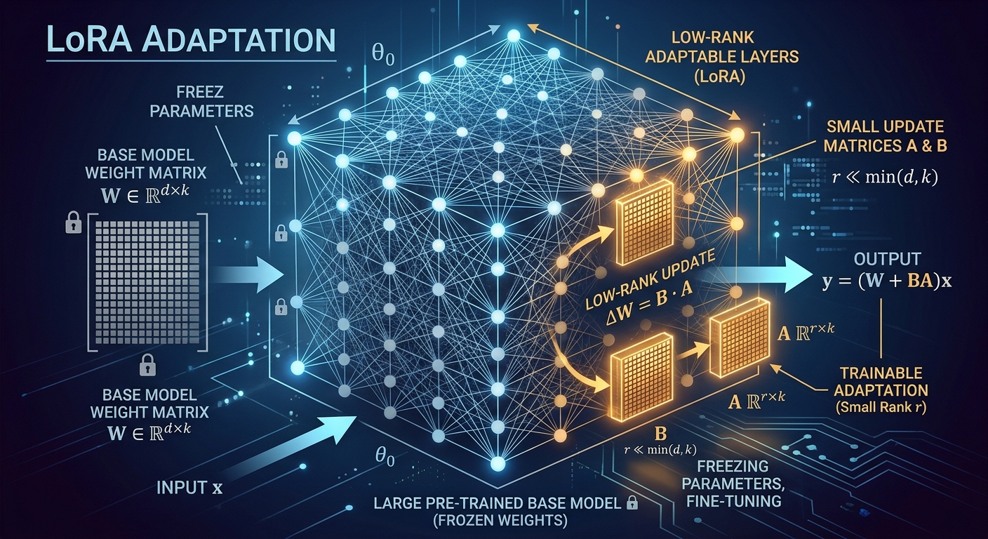
Image: AI Stack Digest Editorial

The local AI landscape in 2026 continues to surprise and empower. While the allure of vast cloud-based models remains, the ability to take a model like Mistral 7B and imbue it with domain-specific intelligence, entirely on your own hardware, is a game-changer. The biggest gotcha nobody talks about enough? Data quality. You can have the latest GPU and perfect LoRA settings, but if your training data is garbage, your fine-tuned model will be, too. It’s an old adage, but it holds: garbage in, garbage out. The real tradeoff against cloud solutions often boils down to scale versus control. Cloud offers infinite scalability at a recurring cost and a trust boundary; local offers finite scale, zero marginal cost, and absolute control over your data and model. What surprised me most during testing for this guide was just how performant 4-bit QLoRA is on a modern 12GB GPU. It’s not just for experimenting anymore; it’s a legitimate path to production for many specialized applications. The barrier to entry for highly customized AI has never been lower, and that’s a truly exciting development for open-source AI.

This article was produced with the assistance of AI tools and reviewed by the AIStackDigest editorial team.